kAIzo: LMs, RNNs, & VAEs for generating kaizo SMM2 levels – World 1-1 LMs

1/nth of Mario 1-1

I took a break from playing Animal Crossing (albeit a short one) so that I could play with the new update to Super Mario Maker 2 (SMM2); the addition of SMB2, and its world creator. I’ve been looking for a new “short-ish” type project to work on while I take a break from other projects, and I wondered whether I could use some form of machine learning to generate levels for SMM2. Also, there’s always more room for learning, and this gave me an opportunity to re-brush up on RNNs (not having used them since I graduated), and work with VAEs.

There are some really awesome levels and I wanted to see if a “sticks and stones” ML model could do any better. Be warned that this method is guaranteed to take much longer than building a level manually. My ultimate goal is to create a “Kaizo” level.

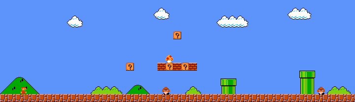
For those who aren’t pro-gamers (like me), SMM2 is essentially an “infinite” Mario game. It has a story line, but its main draw is that players can create their very own levels, in many different styles of the game, using every possible element of the original games and more. This means there’s a lot of factors, features, and other variables to consider, especially across the different game styles; different {enemy, block, power-up, item, building} types. To make this project easier and less time consuming (also constraining it a little), I decided to focus solely on the SMW game style within SMM2.

My intention is to build a simple baseline model to generate levels, followed by a RNN \(\pm\) LSTM, and a VAE. Initially, I was going to dive straight into VAEs, as I’ve recently been studying them, however as I got more familiar with the problem and figured this would be a sequential text-based problem I’d be working on, that I’d first start with simple language models (LMs).

I’ve broken this post into a series as I anticipate it will otherwise be way too long to fit into one post. This first post, aptly named World 1-1, will focus on introduction, data collection/exploration, feature engineering, and building n-gram and Markov Chain LMs.

Also, some “preface” notes; 1) this is just a project worked on solely for a bit of fun and to learn stuff along the way. I have no real interest in PCG, meaning I didn’t spend too long researching the field, except skimming some papers, and so I probably am not making use of existing algorithms and/or methods present in PCG meaning some of my assumptions or paths are likely to be wrong; and 2) because these posts have the potential to be very long, I won’t be explaining things like how a RNN works in detail, instead I’ll assume the reader has some familiarity with the topics presented. The references section at the bottom of the page will contain a bibliography of papers + extra learning & reading materials.

Continue reading “kAIzo: LMs, RNNs, & VAEs for generating kaizo SMM2 levels – World 1-1 LMs”

Nussinov algorithm to predict secondary RNA fold structures

The prediction of secondary RNA structures is an interesting and important problem in bioinformatics. It is by no means at the forefront of the area, but still cool to look at as an introduction to bio(informatics/computation). This post will introduce the Nussinov-Jacobson algorithm for predicting and building secondary fold structures of RNA sequences. It is a dynamic programming algorithm and was one of the first developed for the prediction of RNA structures as RNA combinatorics can be quite involved and expensive. For a recap on dynamic programming, check out this post!

RNA & Nussinov

RNA, DNAs less famous cousin, is in charge of carrying out and transferring the genetic messages set out by DNA to your body for tasks such as protein synthesis. DNA codes and acts as a blueprint for your genetic traits, while the various types of RNA convert that genetic information into useful proteins by transferring the DNA blueprints out of the nucleus and into the ribosome. Both DNA and RNA are pretty cool.

Formally now, we can define RNA as a sequence \(S\), made up of four (nucleotide) bases; \(S \in \{G, C, A, U\}\). These 4 bases come in pairs, known as Watson-Crick pairs, and couple as follow: \(G \leftrightarrow C, \; A \leftrightarrow U\). These pairs are the “strong/stable” base pairs, however, in reality, we also have the coupling of less stable pairs, known as canonical pairs, namely \(G \leftrightarrow U\).

Continue reading “Nussinov algorithm to predict secondary RNA fold structures”

0/1 Knapsack Discrete Optimization w/ Dynamic Programming

The Knapsack problem is one I’ve encountered a handful of times, both in my studies (courses, homework, whatever…), and in real life. Unfortunately, the times I encountered it in a real situation I never had to actually fully solve it – it was more along the lines of, “hey, this is just like the Knapsack problem, but we can work around it”.

I’m currently taking a course on discrete optimization, a field I’ve always thought was cool but never been great at and one which also has a reputation for being particularly hard as you progress deeper. As a way for me to brush up on some basics I thought I’d revisit dynamic programming, an often used technique in solving discrete optimization problems, with the Knapsack problem. The course is very adamant in trying all the different covered algorithms on all problems; for example, if solving Knapsack starts to be too time consuming with DP, use Linear Programming or Branch & Bound with some type of constraint relaxation. To that I say, I will… but I also won’t! I’ll of course try all the algorithms, but since this is a discrete optimization course, I also thought “let me make this even more painful” and try to optimize each algorithm as best I can 🙂

Introduction

The Knapsack problem is actually a combinatorial optimization problem where we need to find an optimal number of objects from a finite set of objects usually based on their properties. It’s an interesting problem as it is both an NP-hard (optimization) and NP-complete (decision) problem that has a pseudo-polynomial algorithm, meaning its worst-case time complexity is polynomial in numeric values of the input. We’ll go through the problem both informally and formally.

Continue reading “0/1 Knapsack Discrete Optimization w/ Dynamic Programming”