The prediction of secondary RNA structures is an interesting and important problem in bioinformatics. It is by no means at the forefront of the area, but still cool to look at as an introduction to bio(informatics/computation). This post will introduce the Nussinov-Jacobson algorithm for predicting and building secondary fold structures of RNA sequences. It is a dynamic programming algorithm and was one of the first developed for the prediction of RNA structures as RNA combinatorics can be quite involved and expensive. For a recap on dynamic programming, check out this post!
RNA & Nussinov
RNA, DNAs less famous cousin, is in charge of carrying out and transferring the genetic messages set out by DNA to your body for tasks such as protein synthesis. DNA codes and acts as a blueprint for your genetic traits, while the various types of RNA convert that genetic information into useful proteins by transferring the DNA blueprints out of the nucleus and into the ribosome. Both DNA and RNA are pretty cool.
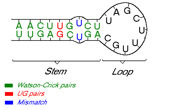
Formally now, we can define RNA as a sequence \(S\), made up of four (nucleotide) bases; \(S \in \{G, C, A, U\}\). These 4 bases come in pairs, known as Watson-Crick pairs, and couple as follow: \(G \leftrightarrow C, \; A \leftrightarrow U\). These pairs are the “strong/stable” base pairs, however, in reality, we also have the coupling of less stable pairs, known as canonical pairs, namely \(G \leftrightarrow U\).
Some types of RNA can form secondary structures by re-pairing up with itself. These secondary structures change the RNA properties drastically. This happens because, unlike DNA, which has a double helix structure, RNA has a single strand structure. Because of this, the RNA sometimes folds in on itself creating these secondary structures. The process of folding can also generate specific patterns or shapes in the RNA structure, such as helixes, loops, bulges, junctions, and pseudoknots. These can occur because of the nature of the fold, or because a nucleotide has had a mismatch pairing. For example, in the image below, \(U\) can not couple with itself, hence creating a small bulge.
There are several approaches to solve the problem of predicting RNA secondary structures, especially with recent developments in the field of bioinformatics and computer science. However, in 1978, a simple yet very effective technique was proposed by Ruth Nussinov et al. which involved a dynamic programming algorithm to predict this secondary structure of an RNA sequence. An extra step is involved with Nussinov’s dynamic programming approach, and that is backtracking. Backtracking allows us to abandon partial solutions as soon as it’s determined that our “in progress” solution can not become a complete solution. If this doesn’t make sense, it soon will upon implementation. The algorithm allows for computing a maximum matching size of \((\sim10^3-10^4)\).
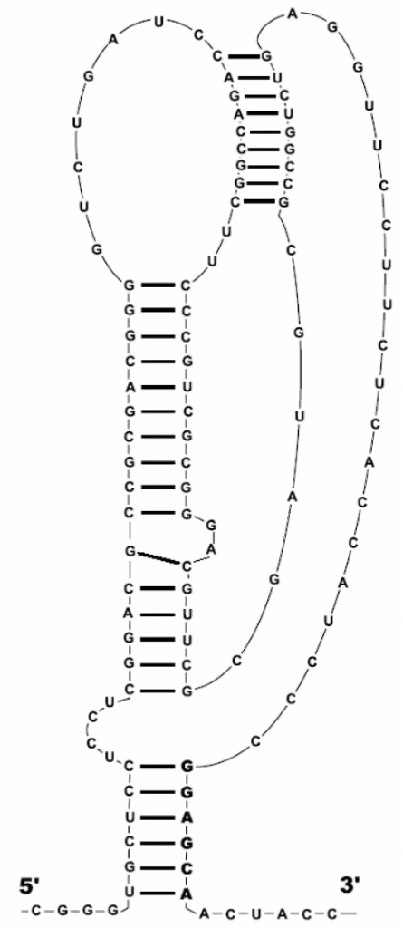
I mentioned that these secondary structures can fold into shapes and patterns, one being a pseudoknot. Pseudoknots are ignored by the Nussinov algorithm as they break down dynamic programming algorithms due to being too complicated to handle and perform backtracking on. In order to enforce this, we will set a minimal loop length in our code so that we do not result in nonsensical base-pairs and loops. Novel algorithms can however support them.
Formalizing the problem once more, we have:
- An RNA molecule as a string, \(S\), where \(S \in \{G, C, A, U\}\) of length \(L = |S|\)
- A secondary RNA structure for \(S\), is a set \(P\) of ordered base pairs, written as \((i, j)\)
- \(j – i > 3\) so as to not have bases too close to each other and avoid pseudoknots
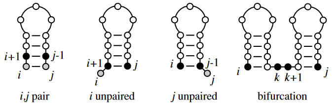
The Nussinov algorithm solves the problem of predicting secondary RNA structures by maximizing base pairs. This also “solves” the problem of predicting non-crossing secondary structures/pseudoknots. This is achieved by assigning a score to our input structure within an \(L \times L\) matrix, \(N_{ij}\). To do this, for every paired set of nucleotides, we give it a score of \(+ 1\), and for others, \(0\). We then attempt to maximize the scores and backtrack on the nucleotides which maximize our overall score. To maximize our base pairs, Nussinov states only 4 possible rules we may use when comparing nucleotides.
The main Nussinov calculations are recursive and calculate the best secondary structures for small subsequences of nucleotides until it reaches larger ones.
Algorithm:
- Add unpaired position \(i\) onto best substructure for subsequence \(i + 1, j\)
- Add unpaired position \(j\) onto best substructure for subsequence \(i, j – 1\)
- Add paired bases \(i – j\) to the best substructure for the subsequence \(i + j, j – 1\)
- Combine two optimal substructures \(i, k\) and \(k + 1, j\)
Therefore, we now have:
\(\gamma(i, j) \; max \begin{cases} \gamma(i + 1, j), \\ \gamma(i, j – 1), \\ \gamma(i + 1, j – 1) + \delta(r_i, r_j), \\ max \{\gamma(i, k) + \gamma(k + 1, j) \} \end{cases}\)
where
\(\delta(i, j) = \begin{cases} 1, & \text{if } x_i – x_j \text{is a pair} \\ 0, & \text{else.} \end{cases}\)
As we’ve now formalized everything, we can begin putting the ideas into practice and writing the relevant code. Let’s get the basic boilerplate functionality going:
import numpy as np

def couple(pair):
    pass

def fill(nm , rna):
    pass

def traceback(nm, rna, fold, i, L):
    pass

def dot_write(rna, fold):
    pass

def init_matrix(rna):
    M = len(rna)

    # init matrix
    nm = np.empty([M, M])
    nm[:] = np.NAN

    # init diaganols to 0
    # few ways to do this: np.fill_diaganol(), np.diag(), nested loop, ...
    nm[range(M), range(M)] = 0
    nm[range(1, len(rna)), range(len(rna) - 1)] = 0

    return nm

if __name__ == "__main__":
    rna = "GGUCCAC" # our RNA sequence
    nm = init_matrix(rna)

    nm = fill(nm, rna)
Ok so we now have some code that returns a matrix of size \(M \times M\), where \(M\) is the length of our RNA sequence, with the first two diagonals set to \(0\) and the rest NaN. Take note we use np.empty rather than np.zeros to save memory, as np.zeros would initialize every value in the matrix to an int. From here, we can begin filling our matrix using Nussinov’s 4 rules. This step is \(\mathcal{O}(L^2), \mathcal{O}(L^3)\) in memory and time respectively.
Just as a less formal explanation, let’s recap how this will work. We’ve initialized the matrix diagonals to \(0\). We now iterate over the matrix, starting at the bottom right, and assign scores of \(+1\) to matching nucleotide pairs. One can even assign scores based on the “strength” of the pair, (i.e, \(\text{A} + \text{U} = 2\)). We do this all the way until we fill the matrix, each time incrementing by \(1\) on a matched pair. We then backtrack with the Nussinov algorithm rules stated above.
def couple(pair):
    """
    Return True if RNA nucleotides are Watson-Crick base pairs
    """
    pairs = {"A": "U", "U": "A", "G": "C", "C": "G"} # ...or a list of tuples...

    # check if pair is couplable
    if pair in pairs.items():
        return True

    return False

def fill(nm, rna):
    """
    Fill the matrix as per the Nussinov algorithm
    """
    minimal_loop_length = 0

    for k in range(1, len(rna)):
        for i in range(len(rna) - k):
            j = i + k

            if j - i >= minimal_loop_length:
                down = nm[i + 1][j] # 1st rule
                left = nm[i][j - 1] # 2nd rule
                diag = nm[i + 1][j - 1] + couple((rna[i], rna[j])) # 3rd rule

                rc = max([nm[i][t] + nm[t + 1][j] for t in range(i, j)]) # 4th rule

                nm[i][j] = max(down, left, diag, rc) # max of all

            else:
                nm[i][j] = 0

    return nm
Running the code together now, we generate a Nussinov matrix given our RNA sequence. Visually, it works something like the figure below. There remains only one step now, and that is the traceback using backtrace (that’s like, 50% of a palindrome). Before I explain how the traceback works, let me explain why we need it. Given our now complete matrix, we need to find the optimal secondary structures. This is based, if you remember, on our base pair maximizations. Essentially, we will be looking at the pairs which contribute the most value to our RNA. To do this, we start at the top right position in the matrix, \(N_{0S}\), where \(S\) is len(rna), and traceback through our maximized base pairs pushing them onto a stack. This traceback is linear in both time and memory.
def traceback(nm, rna, fold, i, L):
    """
    Traceback through complete Nussinov matrix to find optimial RNA secondary structure solution through max base-pairs
    """
    j = L

    if i < j:
        if nm[i][j] == nm[i + 1][j]: # 1st rule
            traceback(nm, rna, fold, i + 1, j)
        elif nm[i][j] == nm[i][j - 1]: # 2nd rule
            traceback(nm, rna, fold, i, j - 1)
        elif nm[i][j] == nm[i + 1][j - 1] + couple((rna[i], rna[j])): # 3rd rule
            fold.append((i, j))
            traceback(nm, rna, fold, i + 1, j - 1)
        else:
            for k in range(i + 1, j - 1):
                if nm[i][j] == nm[i, k] + nm[k + 1][j]: # 4th rule
                    traceback(nm, rna, fold, i, k)
                    traceback(nm, rna, fold, k + 1, j)
                    break

    return fold
We now have our backtraced, optimal secondary RNA structure! There’s only some extra code left which is for output purposes. The general method of output from these algorithms, and to represent RNA sequences, is by writing them out using the dot-bracket notation. Essentially, we have open/closed parenthesis, and dots. An open parenthesis indicates the nucleotide is paired with another ahead of it, a closed parenthesis indicates that a nucleotide is paired with another behind it, and a dot is for unpaired bases. There are other forms of representing RNA, DNA and molecules as strings or graphs however.
def dot_write(rna, fold):
    dot = ["." for i in range(len(rna))]

    for s in fold:
        dot[min(s)] = "("
        dot[max(s)] = ")"

    return "".join(dot)
$ python rna_nussinov.py
     G    G    G    A    A    A    U    C    C
G  0.0  0.0  0.0  0.0  0.0  0.0  1.0  2.0  3.0
G  0.0  0.0  0.0  0.0  0.0  0.0  1.0  2.0  3.0
G  NaN  0.0  0.0  0.0  0.0  0.0  1.0  2.0  2.0
A  NaN  NaN  0.0  0.0  0.0  0.0  1.0  1.0  1.0
A  NaN  NaN  NaN  0.0  0.0  0.0  1.0  1.0  1.0
A  NaN  NaN  NaN  NaN  0.0  0.0  1.0  1.0  1.0
U  NaN  NaN  NaN  NaN  NaN  0.0  0.0  0.0  0.0
C  NaN  NaN  NaN  NaN  NaN  NaN  0.0  0.0  0.0
C  NaN  NaN  NaN  NaN  NaN  NaN  NaN  0.0  0.0
 GGGAAAUCC .((..()))
Done! This was a super fun mini project and I learned a lot about RNA, DNA and other bioinformatics. Every time I researched something new I’d get thrown into a rabbit hole. I enjoy this however! If you’d like to play around with this kind of stuff, I’d recommend checking out “RNAStructure” from MathewsLab research group. It’s not FOSS, but it is free to play with.
You can grab the code for this post directly from here: rna_nussinov.py
Future work
- Support pseudoknots
- Calculate base-pair fold probabilities
- Generate graphviz plot from dot-bracket notation

Resources & References:
Virginia Tech University, CS382
MIT
University of Wisconsin
Algorithms in Bioinformatics
RNA structure analysis
Freiburg RNA Tools
RNA secondary structure prediction